Data Management Cheat Sheet
David D. Liebowitz
EDUC 641: Fall 2024
Setting up project and directory structure
Open your RStudio, create a project and save it. Go to the root directory of the project and create folders named: “Code”, “Data”, “Figures” and “Tables.” Download the life_expectancy.csv dataset and store it in the folder “Data”. Create an R script (or .Rmd) file in the Code folder.
Load relevant packages
# Call one package
library(pacman)
## Warning: package 'pacman' was built under R version 4.1.3# Call multiple packages at once
p_load(tidyverse, here, modelsummary)Read the data in
df <- read.csv(here("data/life_expectancy.csv"))
# There are other packages to read in data that are much faster and more flexible
Extract cases
df <- filter(df, year == 2015)Extract variables
df <- df %>% select(country, status, schooling, life_expectancy)Rename variable
df <- rename(df, region = country)Create a new variable based on existing one(s)
# Replace existing variable
df <- df %>%
      mutate(life_expectancy = round(life_expectancy, digits = 0))
# Create a new one
df <- df %>%
      mutate(life2 = life_expectancy * life_expectancy)
Inspect your data
head(df)## region status schooling life_expectancy life2
## 1 Afghanistan 0 10.1 65 4225
## 2 Albania 0 14.2 78 6084
## 3 Algeria 0 14.4 76 5776
## 4 Angola 0 11.4 52 2704
## 5 Antigua and Barbuda 0 13.9 76 5776
## 6 Argentina 0 17.3 76 5776str(df)## 'data.frame': 183 obs. of 5 variables:
## $ region : chr "Afghanistan" "Albania" "Algeria" "Angola" ...
## $ status : num 0 0 0 0 0 0 0 1 1 0 ...
## $ schooling : num 10.1 14.2 14.4 11.4 13.9 17.3 12.7 20.4 15.9 12.7 ...
## $ life_expectancy: num 65 78 76 52 76 76 75 83 82 73 ...
## $ life2 : num 4225 6084 5776 2704 5776 ...Transform variables, as needed
df$status <- factor(df$status,
                   levels = c(0, 1),
                   labels = c("Developing", "Developed"))
Examine missingness
# One at a time
sum(is.na(df$schooling))
## [1] 10# All at once
sapply(df, function(x) sum(is.na(x)))## region status schooling life_expectancy life2
## 0 0 10 0 0Decide on listwise/pairwise deletion
# In this case, we'll use listwise
df <- filter(df, !is.na(schooling))
Calculate summary statistics
mean(df$life_expectancy)## [1] 71.73988median(df$life_expectancy)## [1] 74sd(df$life_expectancy)## [1] 7.965512summary(df$life_expectancy)## Min. 1st Qu. Median Mean 3rd Qu. Max.
## 51.00 66.00 74.00 71.74 77.00 88.00table(df$status, exclude=NULL)##
## Developing Developed
## 144 29Visualize variables (categorical)
counts <- table(df$status)
barplot(counts)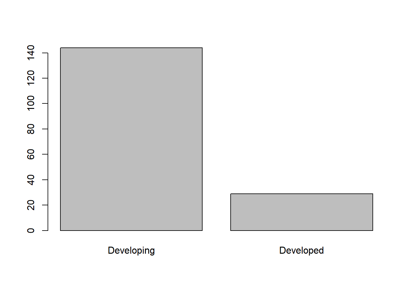
Visualize variables (continuous)
hist(df$life_expectancy)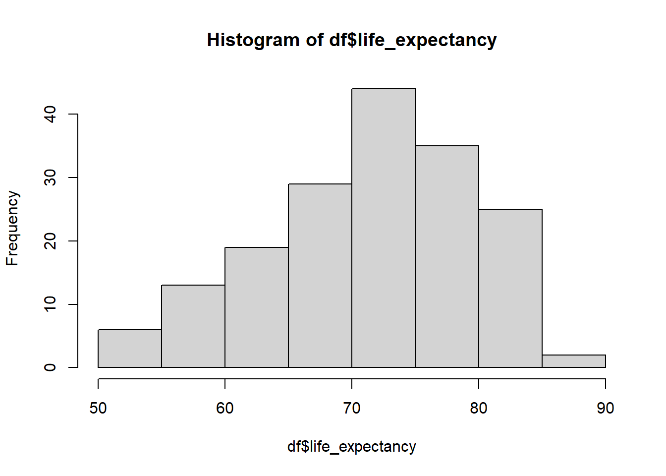
plot(density(df$schooling))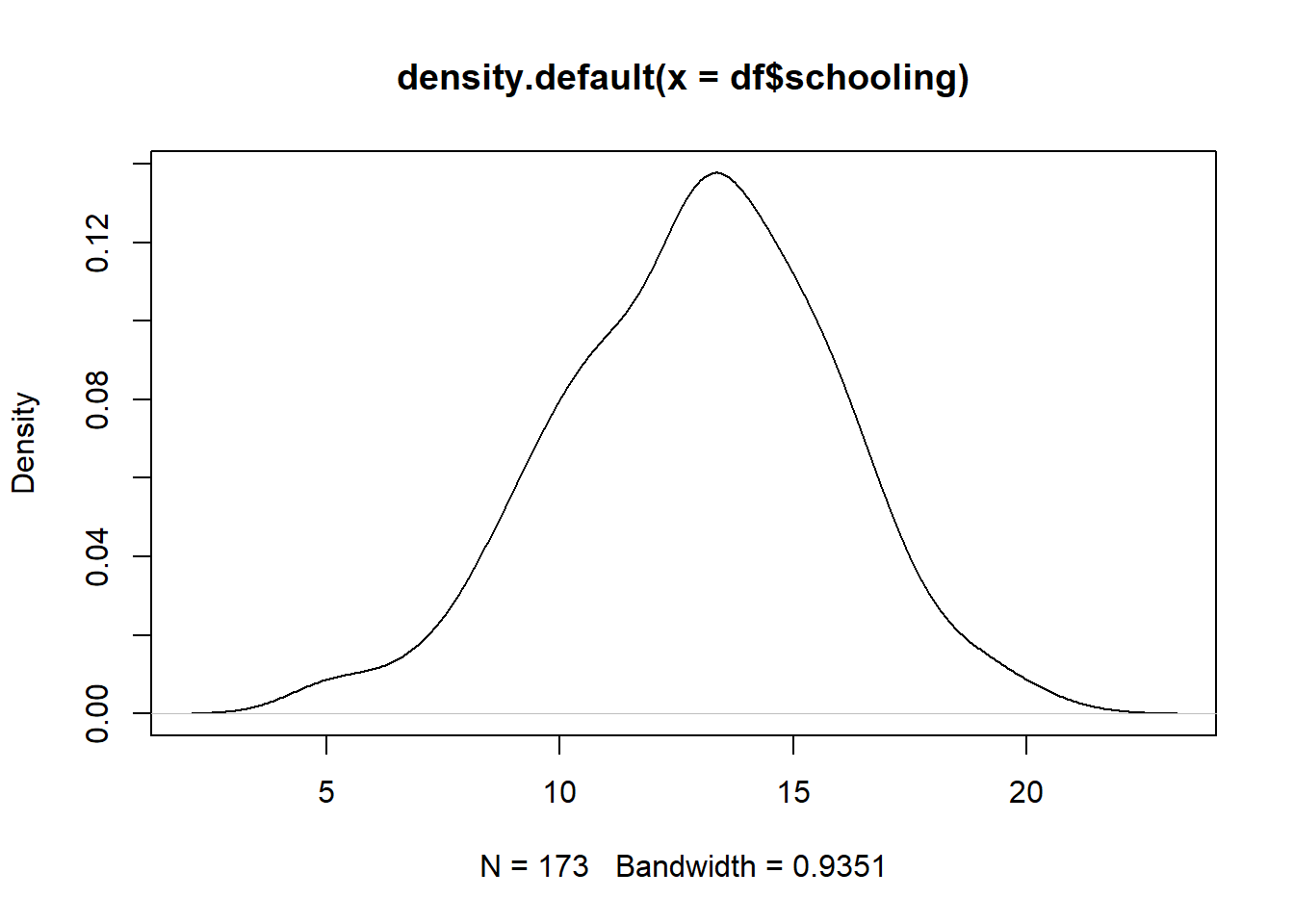
Create descriptive table
desc_df <- select(df, -c(life2))
names(desc_df) <- c("Region", "Status", "Schooling (Yrs)",
                                  "Life Expectancy (Yrs)")

datasummary_skim(desc_df,
                 fun_numeric = list(Mean = Mean, SD = SD, Min = Min,
                                    Median = Median, Max = Max))
## Warning: These variables were omitted because they include more than 50 levels:
## Region.| Mean | SD | Min | Median | Max | |
|---|---|---|---|---|---|
| Schooling (Yrs) | 12.9 | 2.9 | 4.9 | 13.1 | 20.4 |
| Life Expectancy (Yrs) | 71.7 | 8.0 | 51.0 | 74.0 | 88.0 |
| Status | N | % | |||
| Developing | 144 | 83.2 | |||
| Developed | 29 | 16.8 |
Create descriptive table (categorical only)
datasummary_skim(desc_df, type="categorical")## Warning: These variables were omitted because they include more than 50 levels:
## Region.| Status | N | % |
|---|---|---|
| Developing | 144 | 83.2 |
| Developed | 29 | 16.8 |